On real life problems is common to find situations that repeat themselves over and over, i.e. they exhibit a periodic behaviour. Examples of these are: daily variation of the tides and the change
of temperature during a day, among others. On this lesson we will learn to model this type of situations.
|
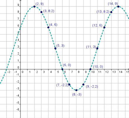
Step 1: Graph the points from the table and identify the Amplitude and the Period. |
Elapsed Hours since 6:00a.m. |
2 |
3 |
4 |
5 |
6 |
7 |
8 |
9 |
10 |
11 |
12 |
13 |
14 |
| Water Level (in feet) |
9 |
8.2 |
6 |
3 |
0 |
-2.2 |
-3 |
-2.2 |
0 |
3 |
6 |
8.2 |
9 |
| 
|
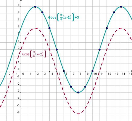
We can see that the points seem to fit a transformed cosine function.
hence, we will obtain the corresponding function if we star from:
y = cos(x)
| Note: Is also valid to use the sine function but the shape formed by the points make us decide to use
the cosine function. |
Amplitude
From the graph we can see that the maximum value is 9 and the minimum value is -3. Hence:
Period
From the graph we see that the cosine function completes a cycle on the interval [2,9]. Hence:
|
|
|
Step 2. Define the steps to follow to build the model. |
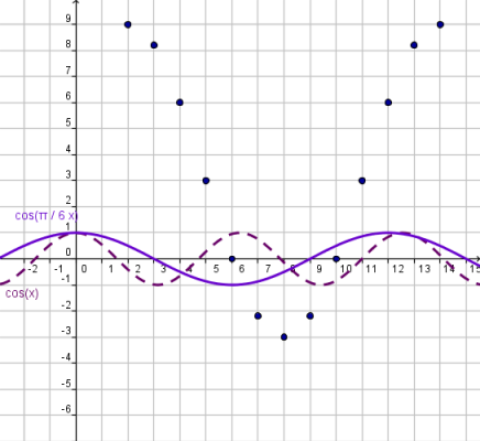
- On the first step we say that we decided to use the cosine function, since it fits better to the actual data.
y = cos(x)
- Change the period of the function y = cos(x) ⇒ y = cos(x) to 12, as identified on step 1.
- Change the amplitude of the function y = cos(kx) y = 6 cos(kx) to 6, as identified on step 1.
- If necessary make an horizontal and/or vertical shift, such that the graph of the model fits the data.
|
Step 3. Include the period on the base function. |
On step 2 we determined that the period of the function is 12.
In the lesson, Period Change of Trigonometric Functions, we learn that if
x is changed to kx, the period changes.
Knowing the period, we can find the value of k, since as we know:
Hence:
From where:
|
 |
|
| Step 4. Include the amplitude in the base function. |
On step 2 we determined the amplitude as 6. Then the function must have an amplitude equal to six.
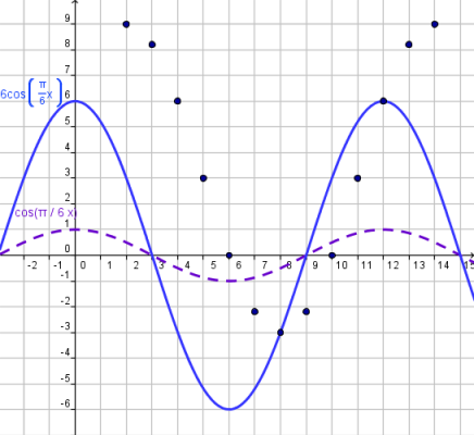
Conclusion: Now we have a model that fits the period and amplitude of our data. Now, we only need to shift the graph to match the data with the graph. |
Step 5. Vertical and Horizontal Shifts. |
We can see that the graph is shifted two units to the right. This means we must subtract 2 to the input.
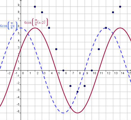 |
We can see that the graph is shifted two units up. This means we must add 3 to the output.
 |
|
|
Step 1: Graph the points from the table and identify the Amplitude and the Period. |
Month |
4 |
5 |
6 |
7 |
8 |
9 |
10 |
11 |
12 |
13 |
14 |
15 |
16 |
| Average Temperature |
63 |
74.5 |
82.9 |
86 |
82.9 |
74.5 |
63 |
51.5 |
43.1 |
40 |
43.1 |
51.5 |
63 |
| 
|
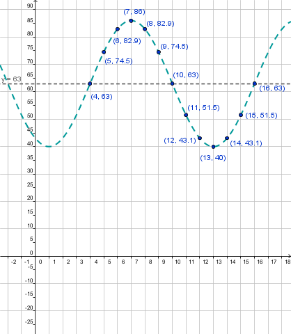
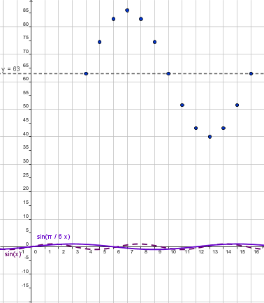
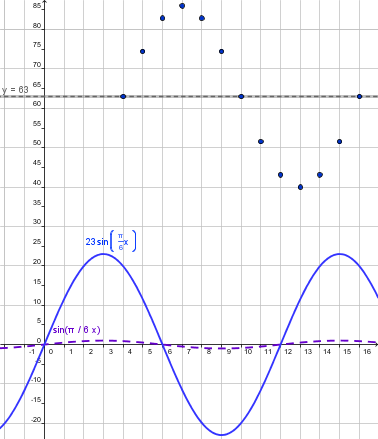
We can see that the points seem to fit a transformed sine function.
hence, we will obtain the corresponding function if we star from::
y = sin(x)
| Note: Is also valid to use the cosine function but the shape formed by the points make us decide to use
the sine function. |
Amplitude
From the graph we can see that the maximum and minimum values are 86 and respectively. Hence:
Period
From the graph we see that the cosine function completes a cycle on the interval [4,16]. Hence:
|
|
|
Step 2: Define the steps to build the model. |
- On the first step we say that we decided to use the sine function, since it fits better to the actual data.
y = sine(x)
- Change the period of the function y = sine(x) ⇒ y = sin(x) to 12, as identified on step 1.
- Change the amplitude of the function y = sine(kx) y = 23 sine(kx) to 23, as identified on step 1.
- If necessary make an horizontal and/or vertical shift, such that the graph of the model fits the data.
|
Step 3: Include the Period on the base function. |
On step 2 we determined that the period of the function is 12.
In the lesson, Period Change of Trigonometric Functions, we learn that if
x is changed to kx, the period changes.
Knowing the period, we can find the value of k since we know
Hence:
Where:
|
With respect to the data the graph looks like:
|
|
| Step 4. Include the Amplitude in the base function. |
On Step 2 the amplitude to be equal to 23. Then the base function must have amplitude 23.
Conclusion: Now we have a model that fits the period and amplitude of our data. Now, we only need to shift the graph to match the data with the graph. |
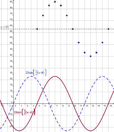
Step 5. Vertical and Horizontal Shifts. |
We see the graph shifted 4 units to the right. In other word we must subtract 4 to the input.
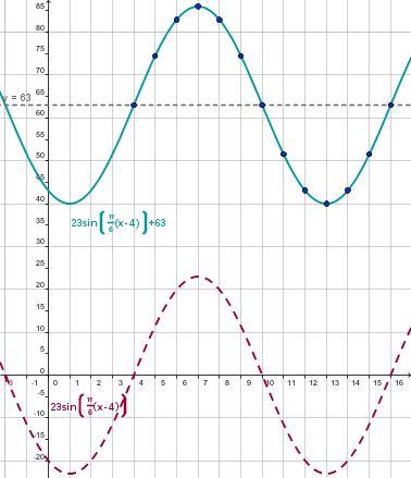
 |
We see the graph shifted 63 units up. So we must add 63 to the output.
 |
|
|
Step 1: Graph the points from the table and identify the Amplitude and the Period. |
Year |
1 |
2 |
3 |
4 |
5 |
6 |
7 |
8 |
9 |
10 |
11 |
12 |
13 |
14 |
15 |
16 |
17 |
| Owls Population |
50 |
61.5 |
71.2 |
77.7 |
80 |
77.7 |
71.2 |
61.5 |
50 |
38.5 |
28.8 |
22.3 |
20 |
22.3 |
28.8 |
38.5 |
50 |
| 
|
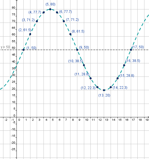
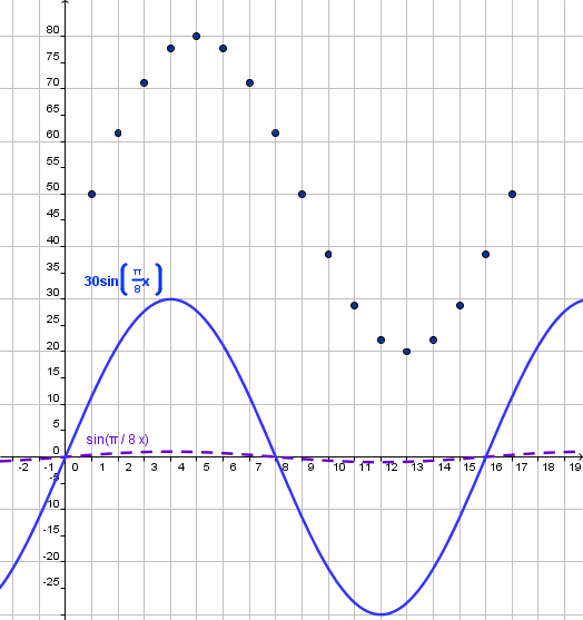
We can see that the points seem to fit a transformed sine function.
hence, we will obtain the corresponding function if we star from::
y = sin(x)
| Note: Is also valid to use the cosine function but the shape formed by the points make us decide to use
the sine function. |
Amplitude
From the graph we can see that the maximum and minimum values are 80 and 20 respectively. Hence:
Period
From the graph we see that the cosine function completes a cycle on the interval [1,17]. Hence:
|
|
|
Step 2: Define the steps to build the model. |
- On the first step we say that we decided to use the sine function, since it fits better to the actual data.
y = sine(x)
- Change the period of the function y = sine(x) ⇒ y = sin(x) to 16, as identified on step 1.
- Change the amplitude of the function y = sine(kx) y = 30 sine(kx) to 30, as identified on step 1.
- If necessary make an horizontal and/or vertical shift, such that the graph of the model fits the data.
|
Step 3: Include the Period on the base function. |
On step 2 we determined that the period of the function is 16.
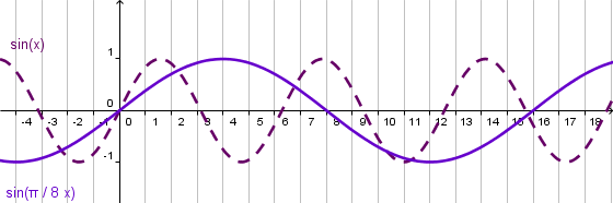
In the lesson, Period Change of Trigonometric Functions, we learn that if
x is changed to kx, the period changes.
Knowing the period, we can find the value of k since we know
Hence:
Where:
|
With respect to the data the graph looks like:

|
|
| Step 4. Include the Amplitude in the base function. |
On Step 2 the amplitude to be 30. Hence the base function must have amplitude equal to 30.
Conclusion: Now we have a model that fits the period and amplitude of our data. Now, we only need to shift the graph to match the data with the graph. |
Step 5. Vertical and Horizontal Shifts. |
We see the graph shifted one unit to the right. In other words we must subtract 1 to the input.
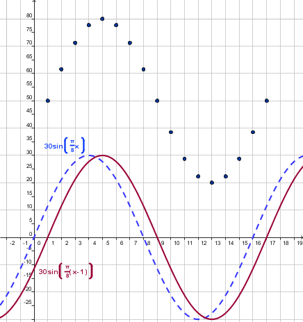 |
We see the graph shifted 50 units up. In other word we must add 50 to the output.
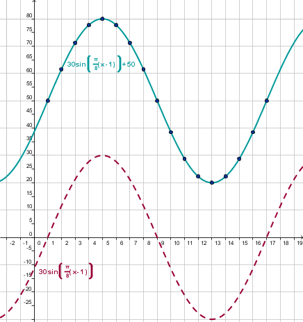 |
|
|
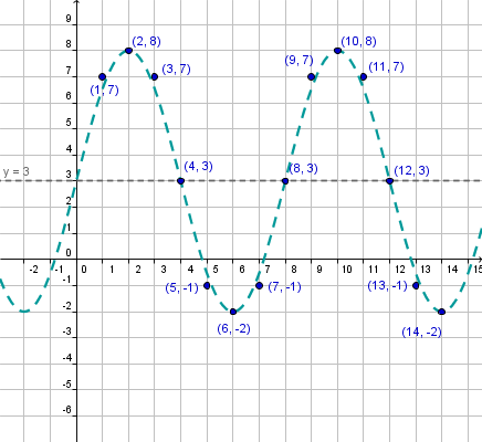
Step 1: Graph the points from the table and identify the Amplitude and the Period. |
Seconds |
1 |
2 |
3 |
4 |
5 |
6 |
7 |
8 |
9 |
10 |
11 |
12 |
13 |
14 |
| Particle Height |
7 |
8 |
7 |
3 |
-1 |
-2 |
-1 |
3 |
7 |
8 |
7 |
3 |
-1 |
-2 |
| 
|
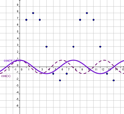
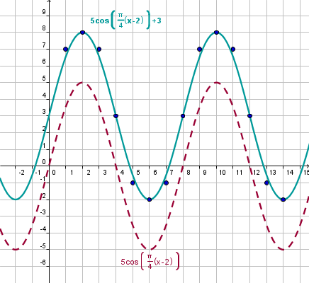
We can see that the points seem to fit a transformed cosine function.
hence, we will obtain the corresponding function if we star from:
y = cos(x)
| Note: Is also valid to use the sine function but the shape formed by the points make us decide to use
the cosine function. |
Amplitude
From the graph we can see that the maximum and minimum values are 8 and -2 respectively. Hence:
Period
From the graph we see that the cosine function completes a cycle on the interval [2,10]. Hence:
|
|
|
Step 2: Define the steps to build the model. |
- On the first step we say that we decided to use the cosine function, since it fits better to the actual data.
y = cos(x)
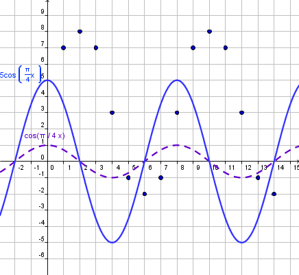
- Change the period of the function y = cos(x) ⇒ y = cos(x) to 8, as identified on step 1.
- Change the amplitude of the function y = cos(kx) y = 5 cos(kx) to 5, as identified on step 1.
- If necessary make an horizontal and/or vertical shift, such that the graph of the model fits the data.
|
Step 3: Include the Period on the base function. |
On step 2 we determined that the period of the function is 5.
In the lesson, Period Change of Trigonometric Functions, we learn that if
x is changed to kx, the period changes.
Knowing the period, we can find the value of k since we know
Hence:
Where:
|
 |
|
| Step 4. Include the Amplitude in the base function. |
On step 2 we determined the amplitude as 5. Then the function must have an amplitude equal to 5.
Conclusion: Now we have a model that fits the period and amplitude of our data. Now, we only need to shift the graph to match the data with the graph. |
Step 5. Vertical and Horizontal Shifts. |
We see that the graph is shifted 2 units to the right. In other words we must subtract 2 from the input.
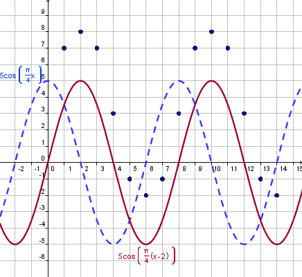 |
We see that the graph is shifted 2 units up. In other words we must add 2 to the output.
 |
|
A research was conducted on the temperature of a city, measures of the average temperature were made from April 2010 to April 2012. The data is registered in the following table:
A research was conducted on a forest populated by owls whose main food resource are mice. The average population of owls for was registered for 13 years as is shown in
the following table:
The following table shows the height of a particle hanging from a spring on a roof per second after the initial movement: