Representing Functions

Objectives

The concepts and techniques presented in this lesson will enable you to:

• Use formulas, graphs, and tables to represent functions
• Determine how to represent a function given a particular situation or question.
• Find function input and output values using formulas, graphs, and tables
• Recognize when a relation represented by a formula, graph, or table is a function

Introduction

In the Functions: An Introduction lesson we visualized functions as machines that process inputs to produce outputs. In previous courses, we have learned to express relationships as formulas, tables and graphs (click here for help). Similarly, the three commonly used forms to represent functions (for now functions are real functions with real number inputs and real number outputs) are formulas, graphs, and tables.

The same function f can often be represented with in different ways. For example, a quadratic function is represented using the formula f (x) = 3x² + 2x − 1 to completely define that function with the formula. While only a finite number of points can be represented, the following table partially represents the same function f.

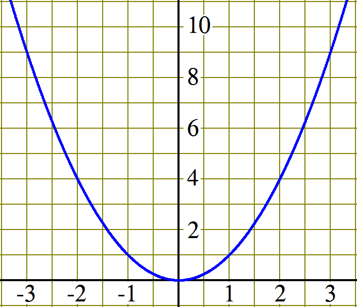
The following graph presents another partial representsion of f with infinite points..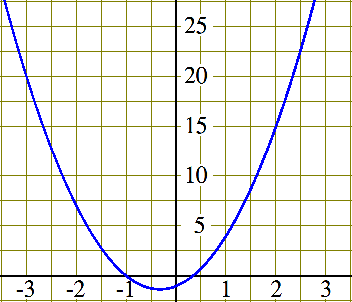

In this section we will summarize how to use these different represntations and explorte the pros and cons associated with their use.

Reading Input and Output Values

Reading input and output values means that given a function represented by a formula, a table, or a graph we should be able to read (find or determine) the corresponnding output value given an input value or the corresponding inputs values given an input value. First, we'll consider a table.

Example 1:

We search through the input (top) row of the table to find 5 , then we read the value just below the 5 from the output (bottom) row: 3.

This time we search through the output (bottom) row of the table to find all the 5s, then we read the value(s) just above the 5s from the input (top) row: 1 and 7.

Now let's work with a function represented by a graph.

Example 2:

If a point (a,b) resides on the graph g that means that when a is input into g, the output is b or that g(a) = b. We can use this to solve the following:

• g(3) = ? or what is the output when 3 is input into g: Solution: As the x coordinate on the graph represents the input into g, we are looking for the oint(s) (3,?) on the graph. By inspection there is only one point with an x coordinate of 3 and that is the point (3,10). Hence g(3) = 10.
• If g(a) = 4, what is the value of a? Or what is the intput when 4 is the output from g: Solution: As the y coordinate on the graph represents the output frp, g, we are looking for the oint(s) (a,4) on the graph. By inspection there is only one point with a y coordinate of 4 and that is the point (6,4). Hence g(6) = 4 and a = 6

Finally, we consider a function represented by a formula.

Example 3:

h(x) = 14 −2x

First we substitute the input value 30.4 for the independent variable x in the formula and then perform the corresponding numerical operations:

h(x) = 14 − 2x

h(30.4) = 14 − 2(30.4)

h(30.4) = 14 − 60.8

h(30.4) = −46.8

First we substitute the output value 30.4 for the result (or dependent variable) h(x) and equate it to the formula. All that remains is to solve the equation for the independent variable x. For some formulas, solving the equation can be very challenging. In this case, the equation is linear:

h(x) = 14 − 2x

30.4 = 14 − 2x

30.4 − 14 = 14 − 2x − 14

16.4 = −2x

$\frac{\mathbf{16}\mathbf{\text{.}}\mathbf{4}}{\mathbf{-}\mathbf{2}}\mathbf{=}\frac{\mathbf{-}\mathbf{2}\mathit{x}}{\mathbf{-}\mathbf{2}}$

−8.2 = x

Click to practice finding function input and output values.

Changing from One Representation to Another

Example 1:

Make a table for the function f  represented by the graph shown below.

To make this table, or any table, from the graphic representation:

1. Find the coordinates of a few points on the graph (points lying on the intersection of gridlines are preferable).
2. Write the x-coordinates and the corresponding y-coordinates of these points in a table.
3. Arrange the table in ascending order of the x-coordinates.

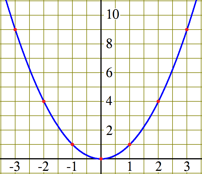
The graph below shows a few points whose coordinates can be read with relative ease and precision.

Reading the coordinates of the marked points from bottom to top, we have (0, 0), (1, 1), (−1, 1), (2, 4), (−2, 4), (3, 9) and (−3, 9). Now, all we have to do is arrange these points in a table in ascending order of the x-coordinates as follows:

The table we produced is only a partial representation of the original graph. Although we should say that the table partially represents the function f , in practice we simply say that the table represents the same function as the graph.

Example 2:

Make a table for the function g represented by the formula g(x) = x³.

To make this table, or any table, from a formula:

1. Evaluate a few small input values (keep the arithmetic simple, unless the function represents a situation in which other input values will be more useful).
2. Write the input values (x-values in this case) and the corresponding results in a table.
3. Arrange the table in ascending order of the x-coordinates.

Now, all we have to do is arrange these input-output pairs in a table in ascending order of the x-coordinates as follows:

The table we produced is only a partial representation of the function defined by the formula x³. Although we should say that the table partially represents the function g, in practice we simply say that the table represents the same function as the formula.

Example 3:

Make a graph for the function g represented by the formula g(x) = x³.

To make a graph from a formula:

1. We begin with a table of values: evaluate a few small input values (always keep the arithmetic simple, unless the function represents a situation that calls for other input values that are more relevant).
2. Draw horizontal and vertical axes with scales that allow all the points in the table to be plotted.
3. Plot the points in the table on the coordinate system drawn.
4. Connect the plotted points in a smooth curve that fits a graph pattern for the formula's type.

We made a small table for the function g(x) = x³ in example 2. If we knew what sort of graph pattern to expect for this formula, seven well-chosen points should be more than enough. However, at this time we only know the pattern for linear formulas and this one is not linear. One of the main objectives in a precalculus course is learning the graph pattern for a few key families of functions. In cases that we don't know the expected pattern, we can make a bigger table to get a better picture of the graph's pattern. The table we made in example 2 used integer input values from −3 to 3. Notice that the table below adds positive intermediate input values rather than expanding the interval. By paying attention to the values in the first small table, we noticed that the results were rotationally symmetric, that is opposite inputs produce opposite outputs. We quickly confirm this observation holds for all x substituting −x in the formula: (−x)³ = −x³. Since the output value 27 is so much bigger than all the others, we want to look at values between 0 and 1. In fact, the smallest changes are around 0, so we'll look at more values close to 0 than 3.

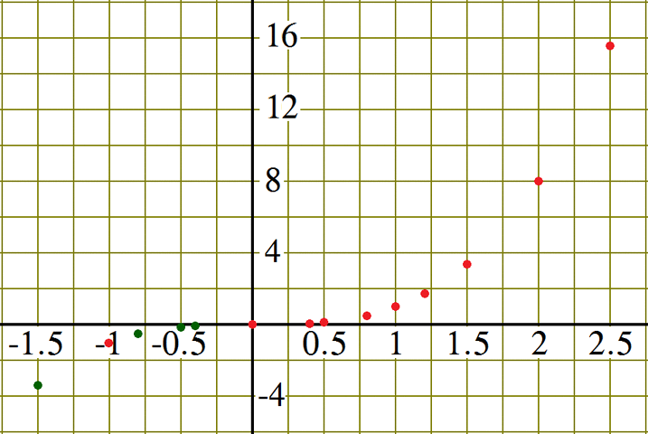
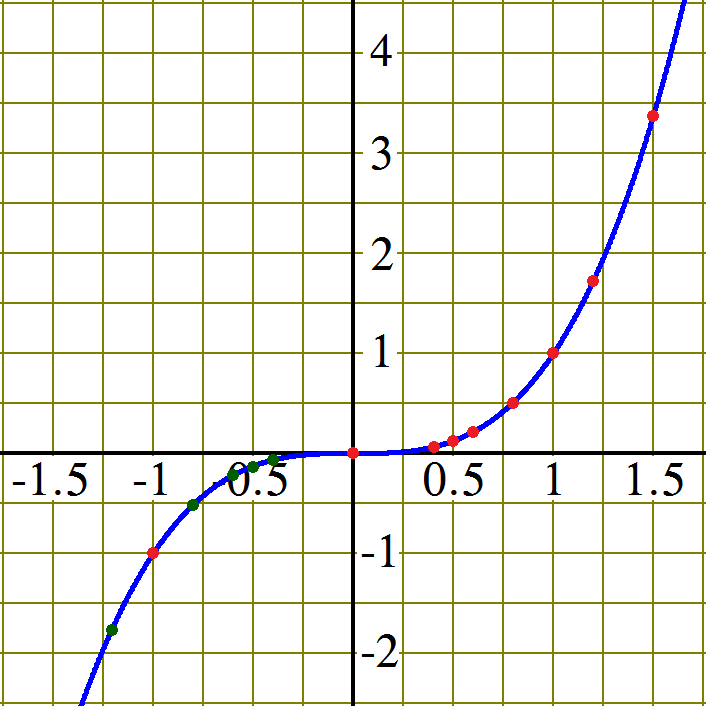
Setting the window so that it includes all of the values in the table is one possibility, but in this case let's try −1.5 ≤ x ≤ 2.5 and −6 ≤ x ≤ 18 and plot the points we can from our table.

The red dots mark the points used from the table and the green dots mark points deduced using the rotational symmetry of the function. All that is left is to connect the points to form a smooth curve.

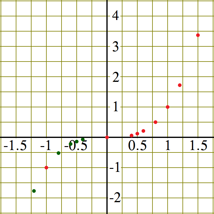
Looking back at the graph we drew, many of the points we plotted ended up very close to the x-axis. While this was expected from the values in the table, we could draw a second graph with a smaller vertical unit to visualize the graphs behavior near x = 0 better. This time we'll use −1.5 ≤ x ≤ 1.5 and −3 ≤ x ≤ 5. We use the same table of values to plot the points. This gives us.

Once again the red dots mark the points used from the table and the green dots mark points deduced using rotational symmetry. Finally we connect the points to form a smooth curve.

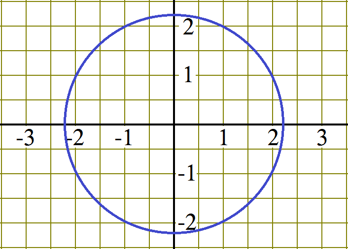
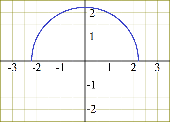
Click to practice evaluating multi-part functions. (See if you can figure it out how they work.)

Interaction: Use the following interactive application to walk through the table, plot, graph process for three basic functions.

Relationship: Function or Not a Function

Some relationships are functions and some are not. A function is a relationship that has a unique output for each input. In the case of a graphical representation, that means that there can be at most one point with any particular x-coordinate. Consider the two graphs shown below and decide which of the two represents a function.

Graph: Function or Not a Function

Not a Function	Function
In the relationship between x and y represented by the graph above, the input value, x = 1 corresponds to two output values, y = 1 and y = −1. Conclusion: So the graph does not represent a function.	In the relationship between x and y represented by the graph above, each input value, x-value, corresponds to only one output value, y-value. There is no vertical line that intersects the graph in more than one point. Conclusion: the graph does represent a function.

Table: Function or Not a Function

A relationship represented by a table is a function if each value in the input row appears only once. (In truth, the input can appear several times, as long as it always appears with the same output value. Yeah, it happens, some tables aren't written efficiently.) Consider the two tables shown below and decide which of the two represents a function.

Formula: Function or Not a Function

Summary

Now that you have successfully completed this lesson, you should be able to:

• Use formulas, graphs, and tables to represent functions
• Find function input and output values using formulas, graphs, and tables
• Recognize when a relation represented by a formula, graph, or table is a function