Piecewise Defined Functions

Objectives

The concepts and techniques presented in this lesson will enable you to:

• Determine the output value of a piecewise defined function for any input value.
• Determine the input values of a piecewise defined function that produce a given output value.
• Sketch the graph of a piecewise defined function.
• Find the domain and range of a piecewise defined function .

Introduction

Not all functions can be represented by a single formula. There is a whole class of functions called piecewise defined functions for which different formulas are used for different inputs. Such functions are used for cab fares, parking lot fees, income taxes, and monthly cell phone charges among others. So-called progressive income tax rates gradually increase as the annual income increases. Consider a machine which calculates the annual income tax owed for a given net income.

The income tax rates in one territory are presented as follows:

• Net income $5,000 or less pay nothing.
• Net income between $5,001 and $22,000, pay 7% of the net income over $5,000.
• Net income between $22,001 and $40,000, pay $1,190 plus 14% of the net income over $22,000.
• Net income between $40,001 and $60,000, pay $3,710 plus 25% of the net income over $40,000.
• More than $60,000 in net income, pay $8,710 plus 33% of the net income over $60,000.

According to this tax rate scheme, the income tax for a resident whose net income was $20,000 for the tax year would be 7% of the net income over $5,000, that is, 0.07 × ($20,000 − $5,000) = $1,050.
The income tax for a resident whose net income was $40,000 for the tax year would be $1,190 plus 14% of the net income over $22,000, that is, $1,190 + 0.14 × ($40,000 − $22,000) = $3,710.
What would the income tax for a resident whose net income was $45,160 for the tax year be?

The graph shown below represents the income tax function corresponding to the rates listed:

$1000

$1000

The abrupt changes in the previous graph make it impossible to write a single simple arithmetic process (a formula) that can be applied to every input. We already calculated the income tax due (the output) for different net incomes (inputs) and we used pretty basic arithmetic. While we didn't follow the same arithmetic process for each net income, we were able to figure out what process to use depending on the net income. We can write a list of those arithmetic processes (formulas) and the net incomes (inputs) for which each of them applies. We could write that list as follows:

$\mathit{T}\mathbf{\left(}\mathit{x}\mathbf{\right)}\mathbf{=}\mathbf{\{}\begin{array}{ccc}\mathbf{0}\hfill & \text{ if }\hfill & \mathit{x}\mathbf{\le }\mathbf{5000}\hfill \\ \mathbf{0}\mathbf{\text{.}}\mathbf{07}\mathbf{(}\mathit{x}\mathbf{-}\mathbf{5000}\mathbf{)}\hfill & \text{ if }\hfill & \mathbf{5000}\mathbf{<}\mathit{x}\mathbf{\le }\mathbf{22000}\hfill \\ \mathbf{0}\mathbf{\text{.}}\mathbf{14}\mathbf{(}\mathit{x}\mathbf{-}\mathbf{22000}\mathbf{)}\mathbf{+}\mathbf{1190}\hfill & \text{ if }\hfill & \mathbf{22000}\mathbf{<}\mathit{x}\mathbf{\le }\mathbf{40000}\hfill \\ \mathbf{0}\mathbf{\text{.}}\mathbf{25}\mathbf{(}\mathit{x}\mathbf{-}\mathbf{40000}\mathbf{)}\mathbf{+}\mathbf{3710}\hfill & \text{ if }\hfill & \mathbf{40000}\mathbf{<}\mathit{x}\mathbf{\le }\mathbf{60000}\hfill \\ \mathbf{0}\mathbf{\text{.}}\mathbf{33}\mathbf{(}\mathit{x}\mathbf{-}\mathbf{60000}\mathbf{)}\mathbf{+}\mathbf{8710}\hfill & \text{ if }\hfill & \mathit{x}\mathbf{>}\mathbf{60000}\hfill \end{array}$

This defines the income tax function in pieces, listing the different formulas to be applied according to the interval to which the input belongs. Literally the function is defined in pieces: one formula for inputs that are less than or equal to 5000, a second for inputs that are greater than 5000 and less than 22000, and so on. We call this a piecewise defined function. When the graphs of functions show abrupt changes like the graph above, we usually need different formulas for different pieces of the function.

The absolute value function is a piecewise defined function:

$\mathbf{\left|}\mathit{x}\mathbf{\right|}\mathbf{=}\mathbf{\{}\begin{array}{ccc}\mathbf{-}\mathit{x}\hfill & \text{ if }\hfill & \mathit{x}\mathbf{<}\mathbf{0}\hfill \\ \mathit{x}\hfill & \text{ if }\hfill & \mathbf{0}\mathbf{\le }\mathit{x}\hfill \end{array}$

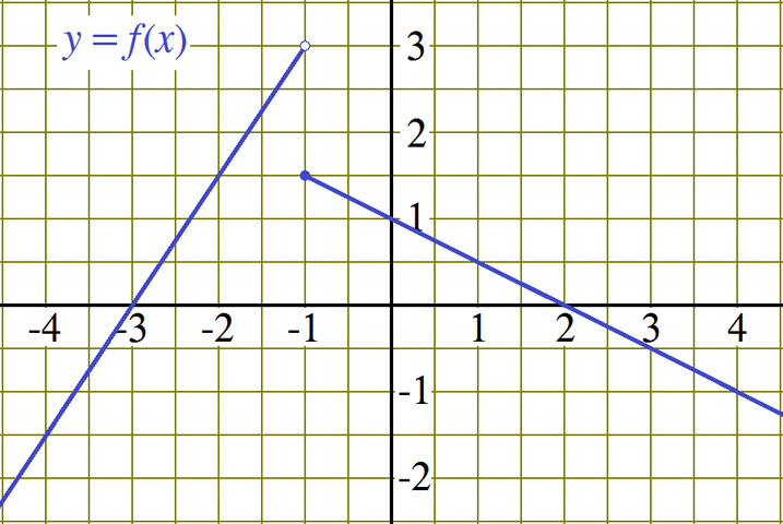
If you are looking at this multi-part definition of the absolute value function and thinking that |x| is always x, then you are assuming that x itself has to be positive. For the definition to include all real numbers, x has to represent negative numbers like −10 as well as positive numbers. So, how do we remove the negative sign if we can't see it?
We don't! We write −x to get the opposite sign. In the case that x = −10, −x = 10. Exactly what we need to get the absolute value. Now, onward and upward.

Graphs

The graph of a piecewise defined function works pretty much the same way as the graph of any other function. The only detail that may be a bit different is the use of oversized circles at certain points on the graph. A filled circle is used to show that the graph includes the corresponding point and that this portion of the graph begins or ends at this particular point. An unfilled circle is used to indicate that a portion of the graph begins or ends at the corresponding point, but does not actually include the point itself. Consider the following graph.

Using the graph above, evaluating the function f  at various inputs yields:
 f (4) = −1,    f (1) = 0.5,  and  f (−2) = 1.5 as usual.

Now, f (−1) = 1.5,    f (−0.98) = 1.49,  and  f (−1.02) = 2.97.

Can you evaluate f (3.5)?

Given that the corresponding portion of the graph is a line segment, the value of f (3.5) should be in the middle of the values for f (3) and f (4). Why?

Using the same graph, we can find the inputs that generate a given output:
 If f (r) = 0, then r = 2 or  −3.
 If f (s) = 1.5, then s = −1 or  −2.
 If f (t) = 3, then t does not exist.

Click to practice evaluating piecewise functions represented by a graph:

Formulas

When evaluating a piecewise defined function, the first is step is to identify which of its sub-formulas should be applied. Each sub-formula is accompanied by the sub-domain to which it is applicable. A well written piecewise defined function will list the sub-formulas in ascending order of sub-domains to facilitate finding the evaluation process. For example, to evaluate g(0) with the following piecewise definition,

$\mathit{g}\mathbf{\left(}\mathit{x}\mathbf{\right)}\mathbf{=}\mathbf{\{}\begin{array}{ccc}\mathbf{2}\mathit{x}\mathbf{+}\mathbf{1}& \text{ if }\hfill & \mathit{x}\mathbf{\le }\mathbf{-}\mathbf{1}\hfill \\ \mathbf{2}{\mathit{x}}^{\mathbf{2}}\mathbf{-}\mathbf{1}& \text{ if }\hfill & \mathbf{-}\mathbf{1}\mathbf{<}\mathit{x}\mathbf{\le }\mathbf{1}\hfill \\ \mathbf{1}\mathbf{-}{\mathit{x}}^{\mathbf{2}}& \text{ if }\hfill & \mathbf{1}\mathbf{<}\mathit{x}\hfill \end{array}$

first we find the input interval to which the input 0 belongs.

It helps to visualize the input intervals and the input on a real number line:

Now that we have identified the input as belonging to the second interval listed in the piecewise definition, −1 < x ≤ 1, we apply the second formula listed:  g(0) = 2(0)² − 1 = −1.

To evaluate g(2), we first find the input interval to which 2 belongs.

Now that we have identified the input as belonging to the third interval listed in the piecewise definition, 1 < x, we apply the third formula listed:  g(2) = 1 − (2)² = −3.

To evaluate g(−1), we find the input interval to which −1 belongs.

This is a little bit more work than the previous cases because −1 is right at the border of the first and second intervals. Since the first interval includes its right hand border, −1 belongs to the first interval listed in the piecewise definition, 1 < x, we apply the first formula listed:  g(−1) = 2(−1) + 1 = −1.

All the input values that produce a given output value for a piecewise defined function can be found by solving an equation for each piece (sub-formula) and selecting the solutions that belong to the sub-domain of that piece. The following shows how to solve the equation g(x) = 0 for the piecewise defined function we have been working with.

Since $\mathit{x}\mathbf{=}\mathbf{-}\frac{\mathbf{1}}{\mathbf{2}}$ does not belong to the first interval x ≤ −1, it is not a solution to the equation g(x) = 0.

Since $\mathbf{\pm }\frac{\sqrt{\mathbf{2}}}{\mathbf{2}}$ do both belong to the second interval −1 < x ≤ 1, both are solutions to the equation g(x) = 0.

Since $\mathbf{\pm }\mathbf{1}$ do not belong to the third interval 1 < x, neither is a solution to the equation g(x) = 0.

So the solutions to the equation g(x) = 0 are $\mathit{x}\mathbf{=}\mathbf{\pm }\frac{\sqrt{\mathbf{2}}}{\mathbf{2}}$.

If we had had a graph of the function g, we might have been able to deduce from the graph which piece could be a 0 and reduce the work to the solving the equation corresponding to the second sub-formula. We'll look at sketching a graph of a piecewise defined function in the next section.

Click to practice evaluating piecewise defined functions from formulas:

Sketching Graphs of Piecewise Defined Functions

To sketch a piecewise defined function's graph, graph each piece over the interval to which it applies (sometimes it can be quicker to graph a piece as if it were the whole formula and then trim to its interval).

• Sketch the graph of each piece (sub-formula) within its sub-domain.
• Carefully mark the endpoints of each sub-graph (the extremes of its sub-domain) to indicate whether the point is part of the graph or simply marks the end or beginning of a sub-graph.

We'll graph the piecewise defined function   $\mathit{f}\mathbf{\left(}\mathit{x}\mathbf{\right)}\mathbf{=}\mathbf{\{}\begin{array}{ccc}\mathbf{1}\mathbf{-}\mathit{x}& \text{ if }\hfill & \mathit{x}\mathbf{<}\mathbf{-}\mathbf{2}\hfill \\ \mathit{x}\mathbf{+}\mathbf{2}& \text{ if }\hfill & \mathbf{-}\mathbf{2}\mathbf{\le }\mathit{x}\mathbf{<}\mathbf{2}\hfill \\ \mathbf{4}\mathbf{-}\mathit{x}& \text{ if }\hfill & \mathbf{2}\mathbf{<}\mathit{x}\hfill \end{array}$  one piece at a time.

First piece: y = 1 − x. This piece is linear, so we just need to plot a couple of the points that belong to the line: (−4, 5) and (0, 1). Connect the points with a line and extend to the edges of the graph. $\mathit{f}\mathbf{\left(}\mathit{x}\mathbf{\right)}\mathbf{=}\mathbf{\{}\begin{array}{ccc}\mathbf{1}\mathbf{-}\mathit{x}& \text{ if }\hfill & \mathit{x}\mathbf{<}\mathbf{-}\mathbf{2}\hfill \\ \mathit{x}\mathbf{+}\mathbf{2}& \text{ if }\hfill & \mathbf{-}\mathbf{2}\mathbf{\le }\mathit{x}\mathbf{<}\mathbf{2}\hfill \\ \mathbf{4}\mathbf{-}\mathit{x}& \text{ if }\hfill & \mathbf{2}\mathbf{<}\mathit{x}\hfill \end{array}$

First Input: The input values for the first piece are −2 < x. So we need to erase everything to the right of x = −2. $\mathit{f}\mathbf{\left(}\mathit{x}\mathbf{\right)}\mathbf{=}\mathbf{\{}\begin{array}{ccc}\mathbf{1}\mathbf{-}\mathit{x}& \text{ if }\hfill & \mathit{x}\mathbf{<}\mathbf{-}\mathbf{2}\hfill \\ \mathit{x}\mathbf{+}\mathbf{2}& \text{ if }\hfill & \mathbf{-}\mathbf{2}\mathbf{\le }\mathit{x}\mathbf{<}\mathbf{2}\hfill \\ \mathbf{4}\mathbf{-}\mathit{x}& \text{ if }\hfill & \mathbf{2}\mathbf{<}\mathit{x}\hfill \end{array}$

First Border: The input values for the first piece do not include x = −2. So we need to mark the end of the line segment with an open circle. $\mathit{f}\mathbf{\left(}\mathit{x}\mathbf{\right)}\mathbf{=}\mathbf{\{}\begin{array}{ccc}\mathbf{1}\mathbf{-}\mathit{x}& \text{ if }\hfill & \mathit{x}\mathbf{<}\mathbf{-}\mathbf{2}\hfill \\ \mathit{x}\mathbf{+}\mathbf{2}& \text{ if }\hfill & \mathbf{-}\mathbf{2}\mathbf{\le }\mathit{x}\mathbf{<}\mathbf{2}\hfill \\ \mathbf{4}\mathbf{-}\mathit{x}& \text{ if }\hfill & \mathbf{2}\mathbf{<}\mathit{x}\hfill \end{array}$

Second Piece: y = x + 2. This piece is also linear, so we plot a couple of the points that belong to the line: (−4, 5) and (0, 1). Connect the points with a line and extend to the edges of the graph. $\mathit{f}\mathbf{\left(}\mathit{x}\mathbf{\right)}\mathbf{=}\mathbf{\{}\begin{array}{ccc}\mathbf{1}\mathbf{-}\mathit{x}& \text{ if }\hfill & \mathit{x}\mathbf{<}\mathbf{-}\mathbf{2}\hfill \\ \mathit{x}\mathbf{+}\mathbf{2}& \text{ if }\hfill & \mathbf{-}\mathbf{2}\mathbf{\le }\mathit{x}\mathbf{<}\mathbf{2}\hfill \\ \mathbf{4}\mathbf{-}\mathit{x}& \text{ if }\hfill & \mathbf{2}\mathbf{<}\mathit{x}\hfill \end{array}$

Second Input: The input values for the second piece are −2 ≤ x < 2. So we need to erase everything new to the left of x = −2 and to the right of x = 2. $\mathit{f}\mathbf{\left(}\mathit{x}\mathbf{\right)}\mathbf{=}\mathbf{\{}\begin{array}{ccc}\mathbf{1}\mathbf{-}\mathit{x}& \text{ if }\hfill & \mathit{x}\mathbf{<}\mathbf{-}\mathbf{2}\hfill \\ \mathit{x}\mathbf{+}\mathbf{2}& \text{ if }\hfill & \mathbf{-}\mathbf{2}\mathbf{\le }\mathit{x}\mathbf{<}\mathbf{2}\hfill \\ \mathbf{4}\mathbf{-}\mathit{x}& \text{ if }\hfill & \mathbf{2}\mathbf{<}\mathit{x}\hfill \end{array}$

Second Borders: The input values for the second piece do include x = −2, but not x = 2. So we need to mark the beginning of the new line segment with a closed circle and the end with an open circle. $\mathit{f}\mathbf{\left(}\mathit{x}\mathbf{\right)}\mathbf{=}\mathbf{\{}\begin{array}{ccc}\mathbf{1}\mathbf{-}\mathit{x}& \text{ if }\hfill & \mathit{x}\mathbf{<}\mathbf{-}\mathbf{2}\hfill \\ \mathit{x}\mathbf{+}\mathbf{2}& \text{ if }\hfill & \mathbf{-}\mathbf{2}\mathbf{\le }\mathit{x}\mathbf{<}\mathbf{2}\hfill \\ \mathbf{4}\mathbf{-}\mathit{x}& \text{ if }\hfill & \mathbf{2}\mathbf{<}\mathit{x}\hfill \end{array}$

Third Piece: y = 4 − x. This piece is also linear, so we plot a couple of the points that belong to the line: (0, 4) and (4, 0). Connect the points with a line and extend to the edges of the graph. $\mathit{f}\mathbf{\left(}\mathit{x}\mathbf{\right)}\mathbf{=}\mathbf{\{}\begin{array}{ccc}\mathbf{1}\mathbf{-}\mathit{x}& \text{ if }\hfill & \mathit{x}\mathbf{<}\mathbf{-}\mathbf{2}\hfill \\ \mathit{x}\mathbf{+}\mathbf{2}& \text{ if }\hfill & \mathbf{-}\mathbf{2}\mathbf{\le }\mathit{x}\mathbf{<}\mathbf{2}\hfill \\ \mathbf{4}\mathbf{-}\mathit{x}& \text{ if }\hfill & \mathbf{2}\mathbf{<}\mathit{x}\hfill \end{array}$

Third Input: The input values for the third piece are 2 < x. So we need to erase everything new to the left of x = 2. $\mathit{f}\mathbf{\left(}\mathit{x}\mathbf{\right)}\mathbf{=}\mathbf{\{}\begin{array}{ccc}\mathbf{1}\mathbf{-}\mathit{x}& \text{ if }\hfill & \mathit{x}\mathbf{<}\mathbf{-}\mathbf{2}\hfill \\ \mathit{x}\mathbf{+}\mathbf{2}& \text{ if }\hfill & \mathbf{-}\mathbf{2}\mathbf{\le }\mathit{x}\mathbf{<}\mathbf{2}\hfill \\ \mathbf{4}\mathbf{-}\mathit{x}& \text{ if }\hfill & \mathbf{2}\mathbf{<}\mathit{x}\hfill \end{array}$

Third Borders: The input values for the third piece do not include x = 2. So we need to mark the beginning of the new line segment with an open circle. $\mathit{f}\mathbf{\left(}\mathit{x}\mathbf{\right)}\mathbf{=}\mathbf{\{}\begin{array}{ccc}\mathbf{1}\mathbf{-}\mathit{x}& \text{ if }\hfill & \mathit{x}\mathbf{<}\mathbf{-}\mathbf{2}\hfill \\ \mathit{x}\mathbf{+}\mathbf{2}& \text{ if }\hfill & \mathbf{-}\mathbf{2}\mathbf{\le }\mathit{x}\mathbf{<}\mathbf{2}\hfill \\ \mathbf{4}\mathbf{-}\mathit{x}& \text{ if }\hfill & \mathbf{2}\mathbf{<}\mathit{x}\hfill \end{array}$ Finally, we have the complete graph of the piecewise function.

The piece by piece method works for sketching the graph of a piecewise defined function, but it involves a lot of erasing. Lets take a more direct approach to sketch the graph of:

$\mathit{g}\mathbf{\left(}\mathit{x}\mathbf{\right)}\mathbf{=}\mathbf{\{}\begin{array}{ccc}\mathbf{-}\mathit{x}& \text{ if }\hfill & \mathit{x}\mathbf{<}\mathbf{0}\hfill \\ {\mathit{x}}^{\mathbf{2}}\mathbf{-}\mathbf{1}& \text{ if }\hfill & \mathbf{0}\mathbf{\le }\mathit{x}\hfill \end{array}$

The first piece y = −x is linear and the second y = x² − 1 is quadratic. So we need a couple of points to be able to plot the first piece and four or five for the second piece. So we'll make a small table that includes the border values for both pieces. Even though only one of the border points actually is part of the graph, the other will help us draw the graph.

Next, we plot the points from the table, carefully marking (0, 0) with an open point.

Now connect the two points on the left with a line segment and extend to the left. Finally connect the five points on the right in a smooth curve and extend to the right until the edge of the graph (In this case the curve reaches the top edge of the graph as we extend to the right.)

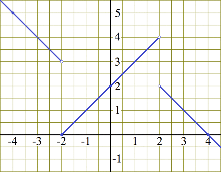
Domain and Range

The domain of a piecewise function defined by a set of formulas is the union of all the sub-domains of those formulas. For example, the domain of

$\mathit{f}\mathbf{\left(}\mathit{x}\mathbf{\right)}\mathbf{=}\mathbf{\{}\begin{array}{ccc}\mathbf{1}\mathbf{-}\mathit{x}& \text{ if }\hfill & \mathit{x}\mathbf{<}\mathbf{-}\mathbf{2}\hfill \\ \mathit{x}\mathbf{+}\mathbf{2}& \text{ if }\hfill & \mathbf{-}\mathbf{2}\mathbf{\le }\mathit{x}\mathbf{<}\mathbf{2}\hfill \\ \mathbf{4}\mathbf{-}\mathit{x}& \text{ if }\hfill & \mathbf{2}\mathbf{<}\mathit{x}\hfill \end{array}$

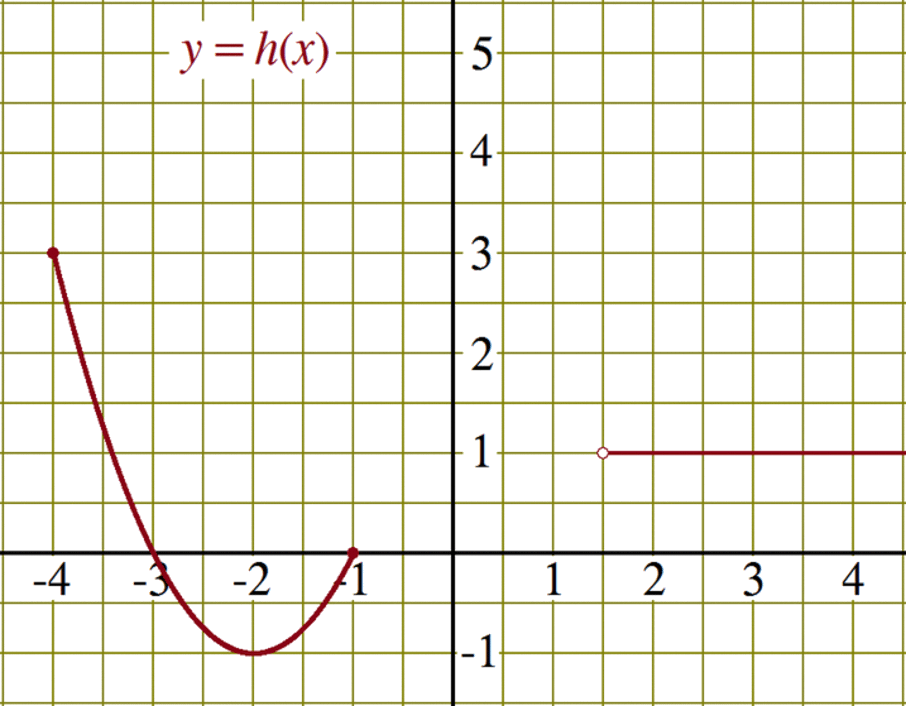
is (−∞, −2) ∪ [−2, 2) ∪ (2, ∞) = (−∞, 2) ∪ (2, ∞) or simply {x | x ≠ 2}.

Similarly, the range of a piecewise function defined by a set of formulas is the union of all the ranges of those formulas over their sub-domains. In the case of the function f  the range is (3, ∞) ∪ [0, 4) ∪ (−∞, 2) = (−∞, ∞).

Having sketched the graph of the function f , finding its domain and range was elementary. Even if we hadn't sketched the graph, all of the sub-formulas were linear so it was just a matter of analyzing the endpoints of each linear piece. Finding the domain and range of piecewise defined functions with non-linear pieces will require more analysis for which we will need to learn more about non-linear functions.

The domain of a piecewise function defined by a graph, like the domain of any function defined by a graph, consists of all the input values (x-coordinates that lie directly above or below points on the graph). For example, the domain of the function h shown in the graph below

is [−4, −1] ∪ (1.5, 4.5].

The range consists of all the output values (y-coordinates that lie directly to the left of to the right of points on the graph). So the range of the function h is [−1, 3].

Notice that the right side of the graph of h continues right up to the edge of the graph. If we assume that we are looking at a partial graph of h and that the graph will continue indefinitely to the right, then the domain would be [−4, −1] ∪ (1.5, ∞). So it is always important to clarify if a graph defines a function or if it is a partial representation that can be assumed to continue in the same direction when it reaches the edge of the window.

Click to practice identifying the domain of piecewise defined functions.	Click to practice identifying the range of piecewise defined functions.

Summary

Now that you have successfully completed this lesson, given a piecewise function defined by a piecewise graph or by formulas in pieces, you should be able to:

• Determine the output value of a piecewise defined function for any input value.
• Determine the input values of a piecewise defined function that produce a given output value.
• Sketch the graph of a piecewise defined function.
• Find the domain and range of a piecewise defined function .